L23L24-QM technique-Software quality prediction

Agenda

• Problem definition
  문제 정의

• Defect prediction process based on machine learning머신러닝 기반 결함 예측 과정

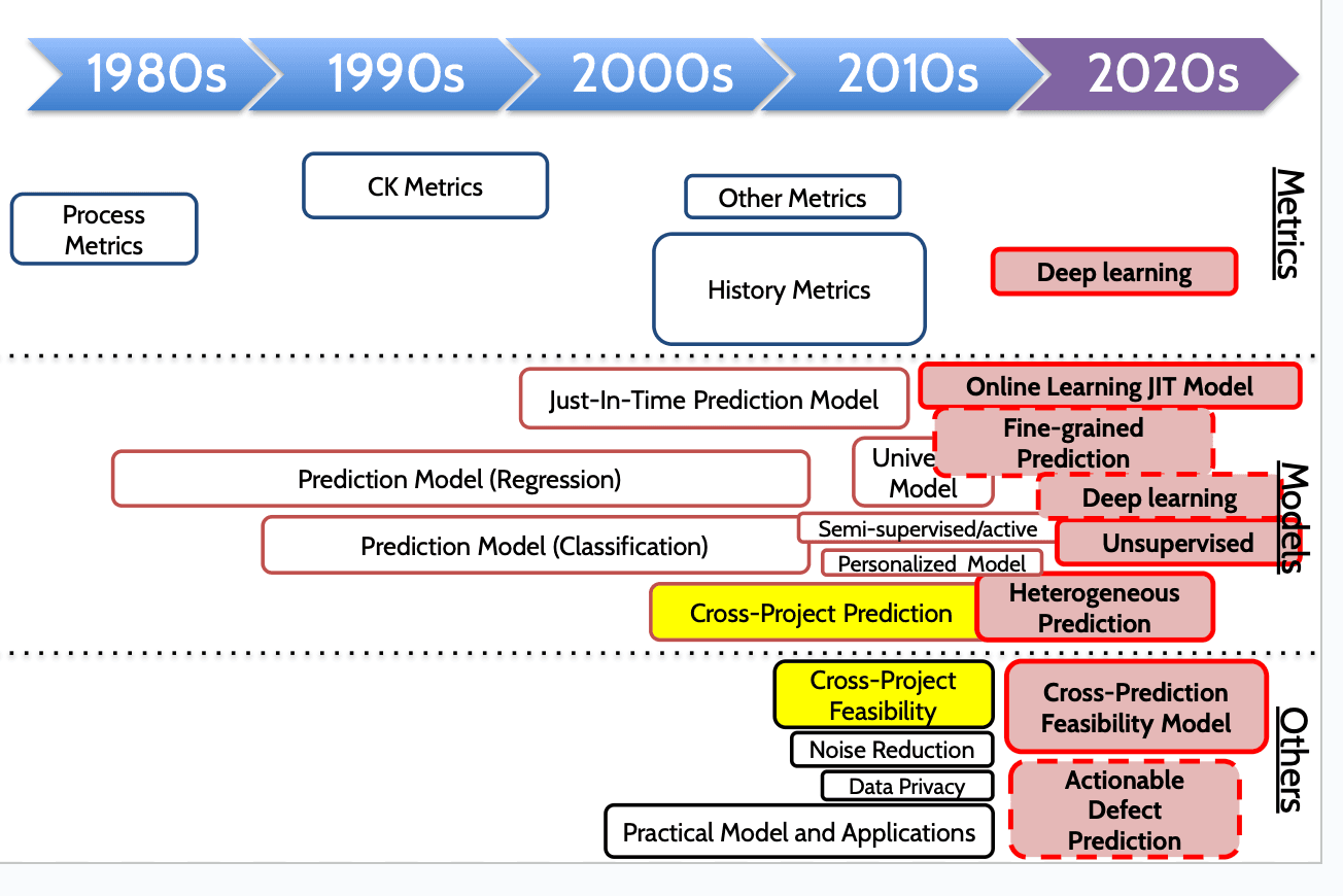
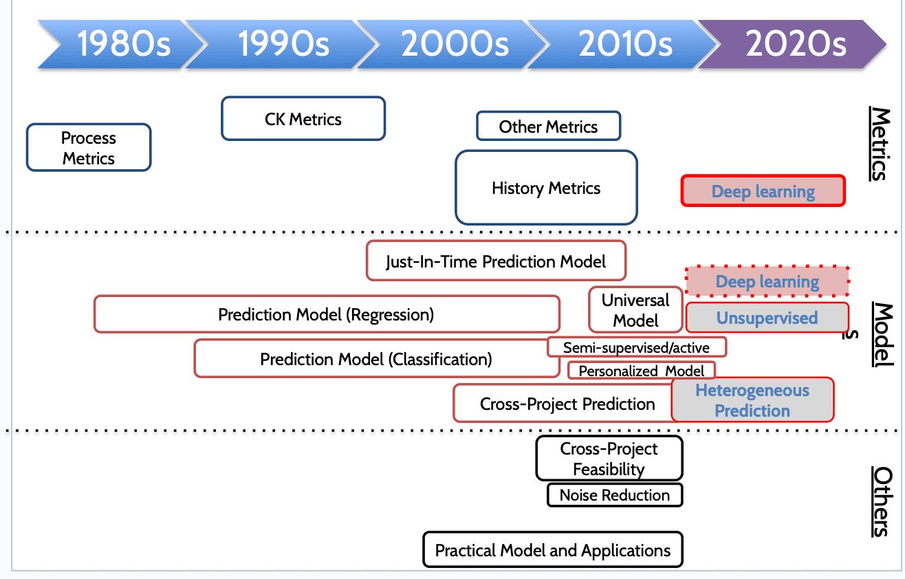
• History of defect prediction studies결함 예측 연구의 역사

• Recent research trends최근 연구 동향

• Current challenges현재의 도전 과제

Motivation

• General question of software defect prediction소프트웨어 결함 예측에 대한 일반적인 질문

  • Can we identify defect-prone entities (source code file, binary, module, change,...) in advance?사전에 결함이 발생하기 쉬운 요소들(소스코드 파일, 바이너리, 모듈, 변경사항 등)을 식별할 수 있는가?

    • # of defects
      결함의 수

    • buggy or clean버그가 많거나 깨끗함

• Why?왜 중요한가?

  • Quality assurance for large software (Akiyama@IFIP’71)대규모 소프트웨어의 품질 보증 (Akiyama@IFIP’71)

  • Effective resource allocation효율적인 자원 분배

    • Testing (Menzies@TSE07)테스트 작업 (Menzies@TSE07)

    • Code review (Rahman@FSE’11)코드 리뷰 작업 (Rahman@FSE’11)

Ground Assumption

• The more complex, the more defect-prone복잡할수록 결함이 발생할 가능성이 높다

Agenda

• Problem definition문제 정의

• Defect prediction process based on machine learning머신러닝 기반 결함 예측 과정

• History of defect prediction studies결함 예측 연구의 역사

• Recent research trends최근 연구 동향

• Current challenges현재의 도전 과제

Defect Prediction Process (Based on Machine Learning)

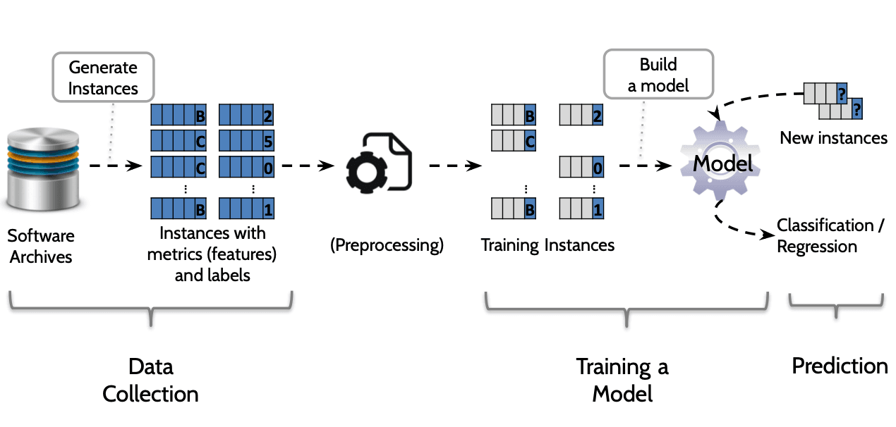
• Data Collection Period데이터 수집 기간

  • Collect Labels레이블 수집(예: buggy vs. clean, 버그 개수)

    • (e.g., buggy vs. clean, # of bugs)

  • Collect Metrics메트릭 수집예: LOC(코드 라인 수)

    • e.g., LOC (lines of code)

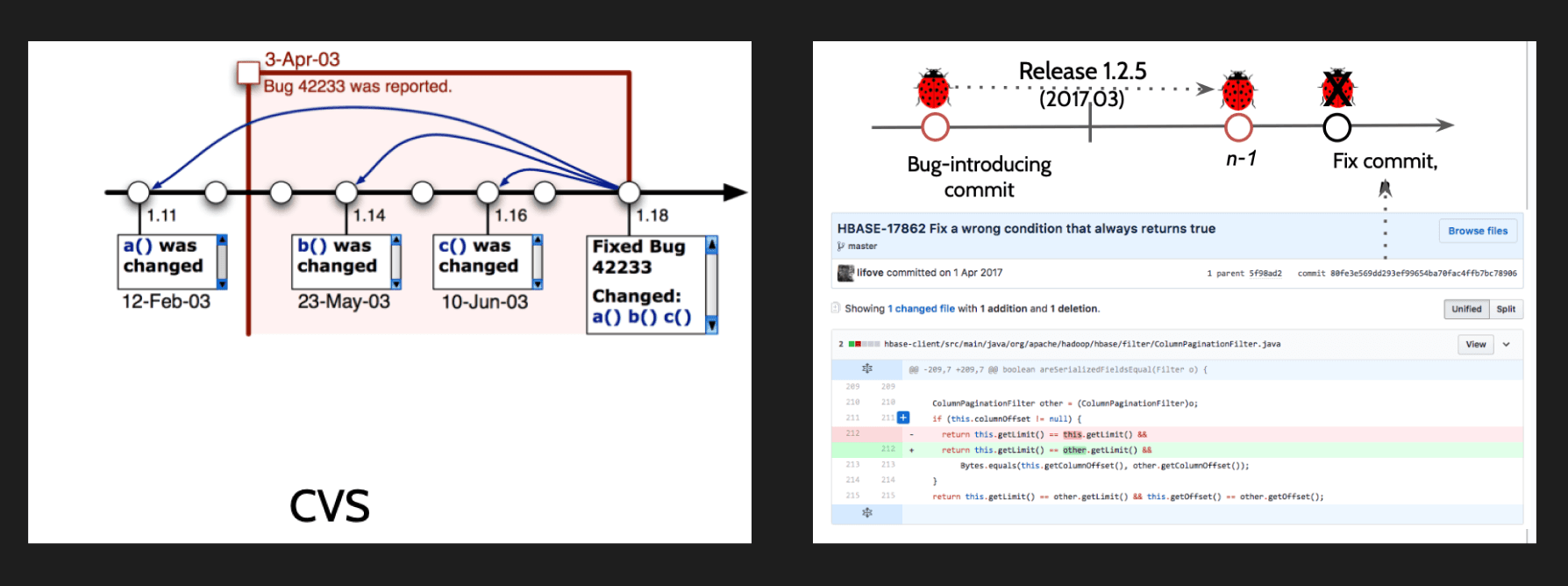
• Bug data for labeling레이블링을 위한 버그 데이터

  • SZZ algorithmSZZ 알고리즘

  • Git BlameGit Blame 도구

• Prediction Model예측 모델

  • Random Forest랜덤 포레스트

  • Support Vector Machine서포트 벡터 머신

  • Logistic Regression로지스틱 회귀

  • J48 Decision TreeJ48 결정 트리

  • Linear Regression선형 회귀

  • ......

Evaluation Measures (classification)

• Measures for binary classification이진 분류를 위한 평가 지표

  • Confusion matrix혼동 행렬

• False positive rate (FPR, PF) = FP / (TN + FP)거짓 양성 비율 = FP / (TN + FP)

• Accuracy = (TP + TN) / (TP + FP + TN + FN)정확도 = (TP + TN) / (TP + FP + TN + FN)

• Precision = TP / (TP + FP)정밀도 = TP / (TP + FP)

• Recall = TP / (TP + FN)재현율 = TP / (TP + FN)

• F-measure = 2 * Precision * Recall / (Precision + Recall)F-점수 = 2 * 정밀도 * 재현율 / (정밀도 + 재현율)

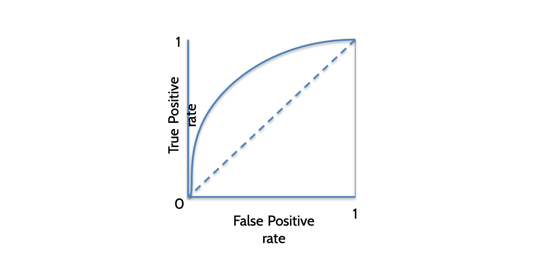
• AUC (Area Under receiver operating characteristic Curve)AUC (수신자 조작 특성 곡선 아래 면적)

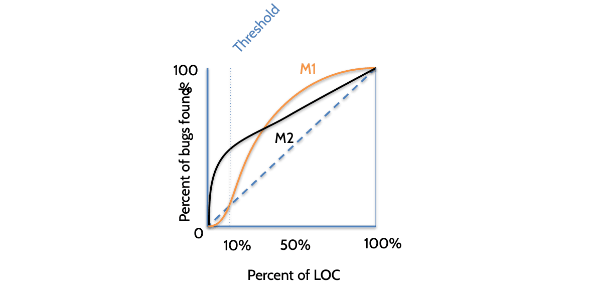
• AUCEC (Area Under Cost Effectiveness Curve)AUCEC (비용 효과 곡선 아래 면적)

Prediction Performance Goal

• Recall vs. Precision재현율 vs. 정밀도

  • Strong predictor criteria강력한 예측기의 기준

  • 70% recall and 25% false positive rate (Menzies@TSE07)재현율 70%, 거짓 양성 비율 25% (Menzies@TSE07)

  • Precision, recall, accuracy ≥ 75% (Zimmermann@FSE09)정밀도, 재현율, 정확도 모두 75% 이상 (Zimmermann@FSE09)

• Cost Effectiveness

  • Effort노력 기준

  • Review 20% of source code and find 80% of bugs소스코드의 20%만 검사해서 80%의 버그를 발견(즉, AUCEC20 = 80%)

Agenda

• Problem definition
  문제 정의

• Defect prediction process based on machine learning머신러닝 기반 결함 예측 과정

• History of defect prediction studies결함 예측 연구의 역사

• Recent research trends최근 연구 동향

• Current challenges현재의 도전 과제

Two Focuses on Defect Prediction

• How much complex is software and its process?소프트웨어와 그 개발 과정이 얼마나 복잡한가?

  • Metrics = (Data)
    메트릭 = (데이터)

  • How can we predict whether software has defects?
    소프트웨어에 결함이 있는지 어떻게 예측할 수 있을까?

  • Models based on the metrics
    메트릭 기반의 예측 모델

Defect Prediction Approaches (1)결함 예측 접근 방식

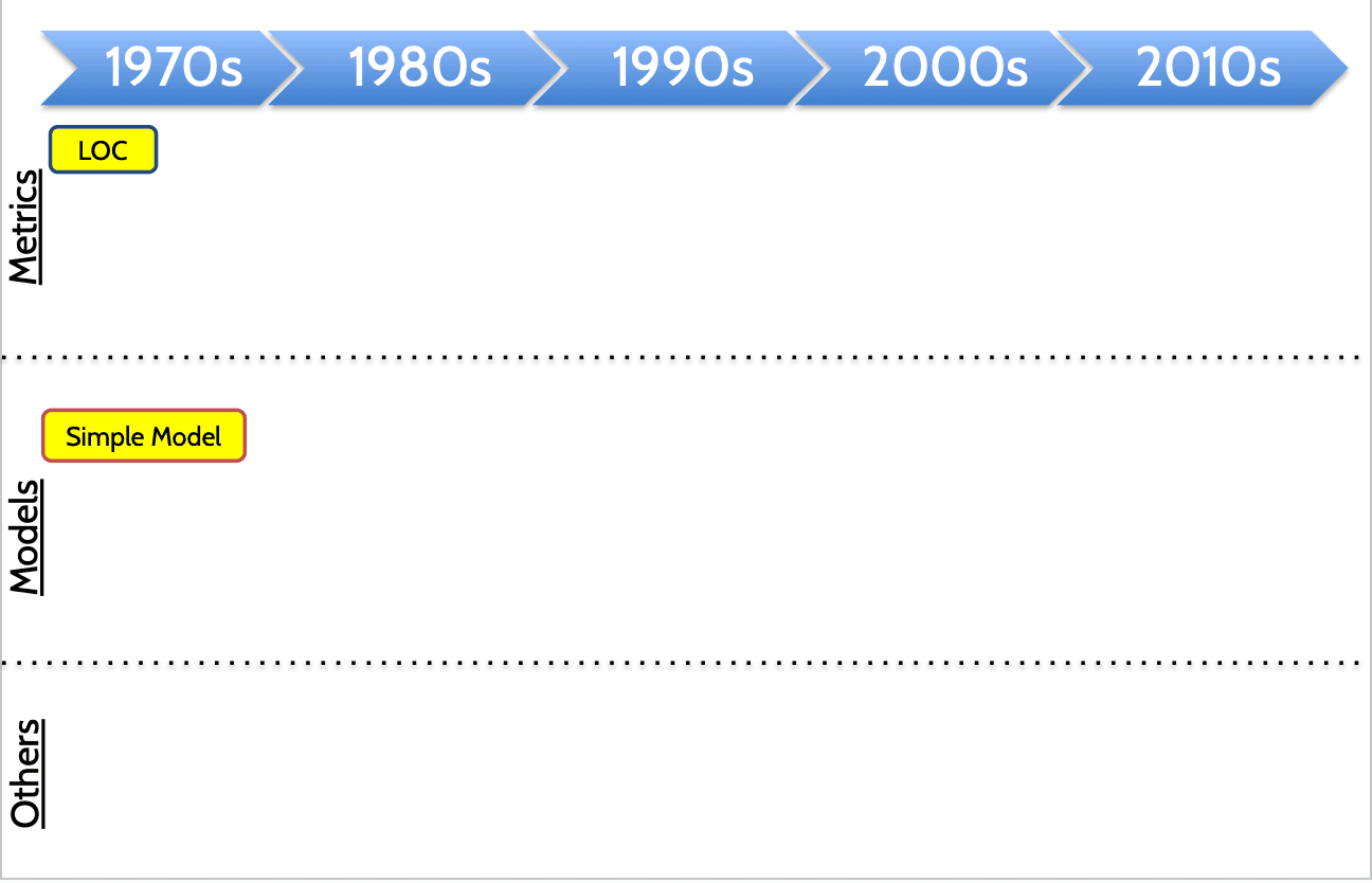
1. Identifying Defect-prone Entities

• Akiyama’s equation (Akiyama@IFIP71) 아키야마의 수식 (Akiyama@IFIP71)

  • # of defects = 4.86 + 0.018 * LOC (=Lines Of Code)결함 수 = 4.86 + 0.018 * LOC (코드 라인 수)

  • 23 defects in 1 KLOKC1 KLOC(1천 줄)당 약 23개의 결함

  • 실제 시스템에서 도출된 수식

  • 코드가 많아질수록 오류가 발생할 수 있다.

• Limitation한계점

  • Only LOC is not enough to capture software complexityLOC만으로는 소프트웨어의 복잡도를 충분히 설명할 수 없다

Defect Prediction Approaches (2)결함 예측 접근 방식

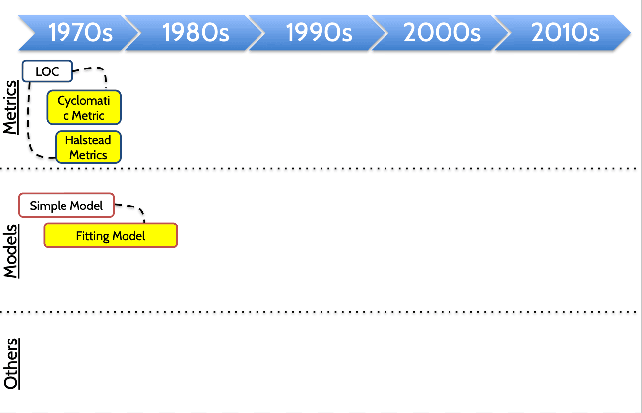
2. Complexity Metrics and Fitting Models

• Cyclomatic complexity metric (McCabe76) 사이클로매틱 복잡도 메트릭 (McCabe76)

  • “Logical complexity” of a program represented in control flow graph제어 흐름 그래프를 통해 나타내는 프로그램의 논리적 복잡도

  • V(G) = #edge – #node + 2
    V(G) = 엣지 수 – 노드 수 + 2

• Halstead complexity metrics (Halsted77)
  할스테드 복잡도 메트릭 (Halsted77)

  • Metrics based on # of operators and operands
    연산자와 피연산자 수를 기반으로 한 메트릭

  • Volume = N * log2n
    볼륨 = N * log2(n)

  • # of defects = Volume / 3000
    결함 수 = 볼륨 / 3000

• Limitation한계점

  • Do not capture complexity (amount) of change.
    변경의 양이나 복잡도를 포착하지 못한다

  • Just fitting models but not prediction models in most of studies conducted in 1970s and early 1980s
    대부분의 1970~80년대 연구는 예측 모델이 아니라 적합 모델이었다

    • Correlation analysis between metrics and # of defects
      메트릭과 결함 수 간의 상관관계 분석

      • By linear regression models
        선형 회귀 모델을 통해 분석

    • Models were not validated for new entities (modules).
      모델이 새로운 모듈에 대해 검증되지 않았다

Defect Prediction Approaches (3)결함 예측 접근 방식

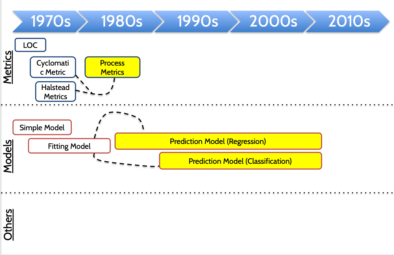
Regression Model회귀 모델

• Shen et al.’s empirical study (Shen@TSE85) 션 외 연구진의 실증 연구 (Shen@TSE85)

  • Linear regression model선형 회귀 모델

  • Validated on actual new modules실제 신규 모듈에 대해 검증됨

  • Metrics사용된 메트릭

    • Halstead, # of conditional statements할스테드, 조건문 수

    • Process metrics프로세스 메트릭

      • Delta of complexity metrics between two successive system versions두 연속된 시스템 버전 간의 복잡도 지표의 차이

  • Measures측정 항목

    • Between actual and predicted # of defects on new modules신규 모듈에서의 실제 vs 예측된 결함 수 비교

      • MRE (Mean magnitude of relative error)상대 오차 평균

        • average of (D - D’)/D for all modules전체 모듈에 대해 (D - D') / D의 평균

          • D: actual # of defectsD: 실제 결함 수

          • D’: predicted # of defectsD’: 예측 결함 수

        • MRE = 0.48

Classification Model

• Discriminative analysis by Munson et al. (Munson@TSE92) 먼슨 외 연구진의 판별 분석 (Munson@TSE92)

  • Logistic regression로지스틱 회귀

  • High risk vs. low risk modules고위험 vs. 저위험 모듈 분류

  • Metrics사용된 메트릭

    • Halstead and Cyclomatic complexity metrics할스테드와 사이클로매틱 복잡도 메트릭

  • Measure측정 항목

    • Type I error: False positive rate1종 오류: 거짓 양성 비율

    • Type II error: False negative rate2종 오류: 거짓 음성 비율

• Result결과

  • Accuracy: 92% (6 misclassification out of 78 modules)정확도: 92% (78개 중 6개 오분류)

  • Precision: 85%정밀도: 85%

  • Recall: 73%재현율: 73%

  • F-measure: 88%F-점수: 88%

Defect Prediction (Based on Machine Learning)

• Limitations한계점

  • Limited resources for process metrics

  • 프로세스 메트릭을 위한 자원이 제한됨

    • Error fix in unit testing phase was conducted informally by an individual developer (no error information available in this phase). (Shen@TSE85)단위 테스트 단계에서의 오류 수정은 개인 개발자에 의해 비공식적으로 수행되어 오류 정보가 없음 (Shen@TSE85)

  • Existing metrics were not enough to capture complexity of object-oriented (OO) programs.기존 메트릭만으로는 객체 지향 프로그램의 복잡도를 포착하기 어려움

  • Helpful for quality assurance team but not for individual developersQA 팀에게는 유용하지만, 개별 개발자에게는 도움이 되지 않음

Defect Prediction Approaches (4)결함 예측 접근 방식

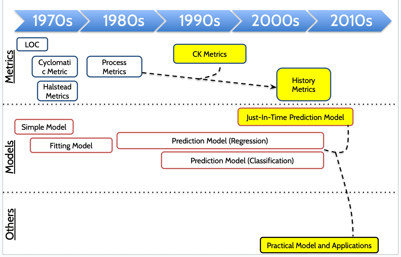
Risk Prediction of Software Changes (Mockus@BLTJ00) 소프트웨어 변경의 위험 예측 (Mockus@BLTJ00)

• Logistic regression로지스틱 회귀

• Change metrics변경 메트릭

  • LOC added/deleted/modified추가/삭제/수정된 코드 라인 수

  • Diffusion of change변경의 확산 범위

  • Developer experience개발자의 경험

• Result결과

  • Both false positive and false negative rate: 20% in the best case거짓 양성률과 거짓 음성률 모두 최선의 경우 20%

• Advantage장점

  • Show the feasible model in practice실제 적용 가능한 모델을 제시

• Limitation한계

  • Conducted 3 times per week주 3회 실행됨

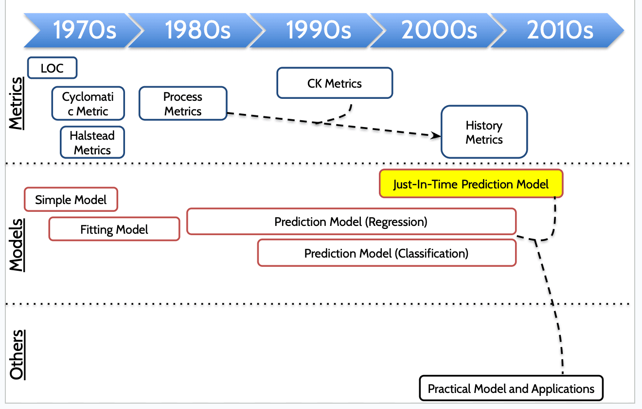
  • Not fully Just-In-Time완전한 실시간 모델은 아님

  • Validated on one commercial system (5ESS switching system software)하나의 상용 시스템(5ESS 교환 시스템 소프트웨어)에서만 검증됨

BugCache (Kim@ICSE07) 버그캐시 (Kim@ICSE07)

• Maintain defect-prone entities in a cache결함 발생 가능성이 높은 파일들을 캐시에 저장

• Approach접근 방식

• Result결과

  • Top 10% files account for 73-95% of defects on 7 systems상위 10%의 파일들이 전체 결함의 73~95%를 차지 (7개 시스템 기준)

• Advantages
  장점

  • Cache can be updated quickly with less cost. (c.f. static models based on machine learning)
    캐시는 머신러닝 기반의 정적 모델에 비해 적은 비용으로 빠르게 갱신할 수 있다.

  • Just-In-Time: always available whenever QA teams want to get the list of defect-prone entities
    JIT(Just-In-Time): QA 팀이 결함 가능성이 높은 항목 목록이 필요할 때마다 항상 즉시 사용 가능하다.

• Limitations
  제한 사항

  • Cache is not reusable for other software projects.캐시는 다른 소프트웨어 프로젝트에 재사용할 수 없다.

  • Designed for QA teamsQA 팀을 위해 설계되었다.

    • Applicable only in a certain time point after a bunch of changes (e.g., end of a sprint)여러 변경 이후 특정 시점(예: 스프린트 종료 시)에만 적용 가능하다.

    • Still limited for individual developers in development phase개발 단계에 있는 개별 개발자에게는 여전히 적용이 제한적이다.

Change Classification (Kim@TSE08) 변경 분류 모델 (Kim@TSE08)

• Classification model based on SVM서포트 벡터 머신(SVM) 기반 분류 모델

• About 11,500 features|약 11,500개의 피처 사용

  • Change metadata such as changed LOC, change count변경된 LOC, 변경 횟수 등의 메타데이터

  • Complexity metrics복잡도 메트릭

  • Text features from change log messages, source code, and file names변경 로그, 소스코드, 파일명에서 추출된 텍스트 특징

• Results결과

  • 78% accuracy and 60% recall on average from 12 open-source projects12개 오픈소스 프로젝트에서 평균 정확도 78%, 재현율 60%

• Limitations한계

  • Heavy model (11,500 features)매우 많은 피처 수로 인해 무거운 모델

  • Not validated on commercial software products.상용 소프트웨어에서 검증되지 않음

Follow-up Studies후속 연구들

• Studies addressing limitations기존 한계를 보완한 연구들

  • “Reducing Features to Improve Code Change-Based Bug Prediction” (Shivaji@TSE`13)코드 변경 기반 결함 예측에서 피처 수를 줄여 성능 개선

    • With less than 10% of all features, buggy F-measure is 21% improved.전체 피처의 10% 미만으로 F-measure가 21% 향상됨

  • “Software Change Classification using Hunk Metrics” (Ferzund@ICSM`09)헝크 메트릭을 이용한 변경 분류

    • 27 hunk-level metrics for change classification변경 분류를 위한 27개 헝크 수준 메트릭

    • 81% accuracy, 77% buggy hunk precision, and 67% buggy hunk recall정확도 81%, 결함 헝크 정밀도 77%, 재현율 67%

  • “A large-scale empirical study of just-in-time quality assurance” (Kamei@TSE13)대규모 실증 연구를 통한 실시간 품질 보증 분석

    • 14 process metrics (mostly from Mockus00)14개의 프로세스 메트릭 사용 (대부분 Mockus`00 기반)

    • 68% accuracy, 64% recall on 11 open-source and commercial projects11개 오픈소스 및 상용 프로젝트에서 정확도 68%, 재현율 64%

  • “An Empirical Study of Just-In-Time Defect Prediction Using Cross-Project Models” (Fukushima@MSR`14)크로스 프로젝트 모델을 활용한 실시간 결함 예측 연구

    • Median AUC: 0.72AUC 중앙값: 0.72

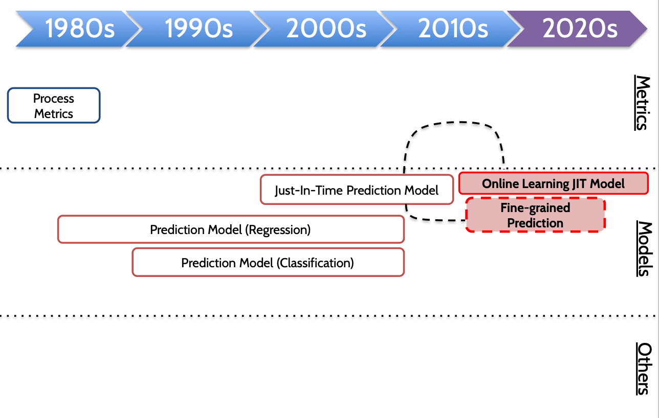
Challenges of JIT modelJIT(Just-In-Time) 모델의 도전 과제

• Practical validation is difficult실제 적용 검증이 어렵다

  • Just 10-fold cross validation in current literature현존 연구들은 대부분 10겹 교차검증에 한정됨

  • Require validation on real scenario실제 시나리오 기반의 검증 필요

  • e.g., online machine learning예: 온라인 머신러닝

• Still difficult to review huge change'대규모 변경에 대한 검토는 여전히 어려움

  • Fine-grained prediction within a change변경 내에서의 세밀한 예측

    • e.g., Line-level prediction예: 라인 단위 예측

Next Steps of Defect Prediction (1)결함 예측의 다음 단계

Defect Prediction Approaches (5)결함 예측 접근 방식

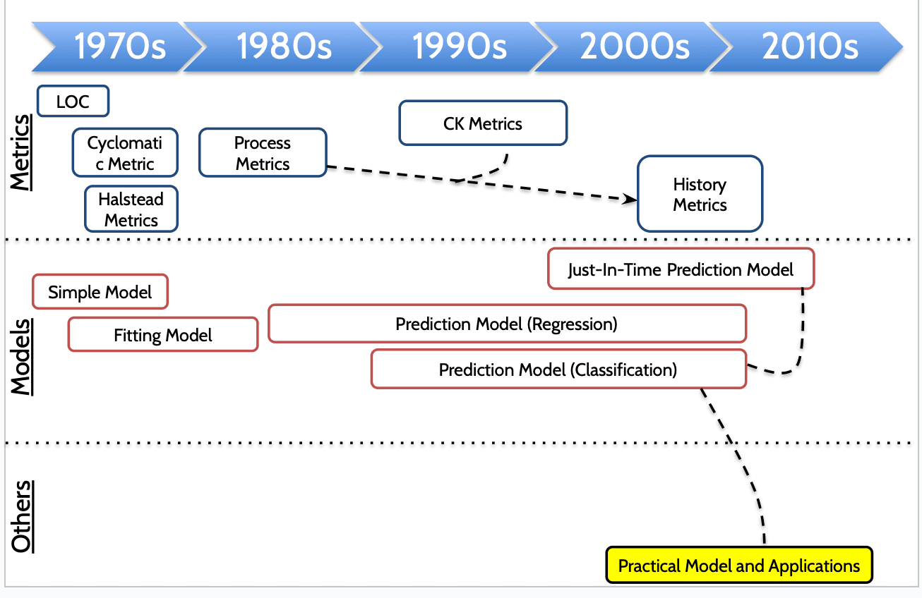
Defect Prediction in Industry산업 현장에서의 결함 예측

• “Predicting the location and number of faults in large software systems” (Ostrand@TSE05)대규모 소프트웨어 시스템에서 결함 위치 및 수 예측 (Ostrand@TSE05)

  • Two industrial systems2개 상용 시스템 대상

  • Recall 86%재현율 86%

  • 20% most fault-prone modules account for 62% faults결함 발생 가능성이 높은 상위 20% 모듈이 전체 결함의 62%를 차지

Case Study for Practical Model실제 적용 모델에 대한 사례 연구

• “Does Bug Prediction Support Human Developers? Findings From a Google Case Study” (Lewis@ICSE`13)결함 예측이 실제로 개발자에게 도움이 되는가? (Google 사례 기반)

  • No identifiable change in developer behaviors after using defect prediction model결함 예측 모델 사용 이후, 개발자 행동에 명확한 변화 없음

• Required characteristics but very challenging필수적이지만 구현이 매우 어려운 특성

  • Actionable messages / obvious reasoning행동 유도형 메시지 / 명확한 근거 제공

Next Steps of Defect Prediction (2)결함 예측의 다음 단계

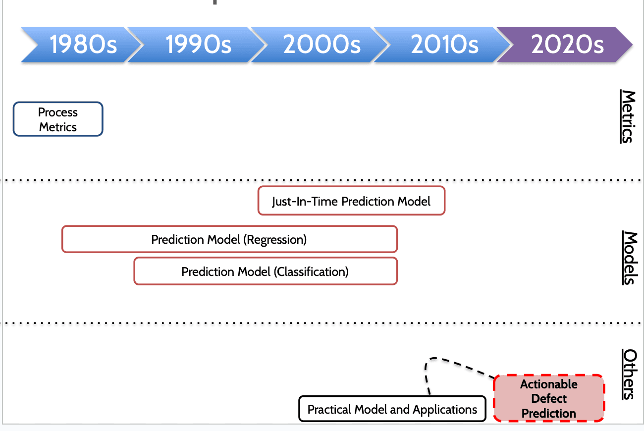
Defect Prediction Approaches (6)결함 예측 접근 방식

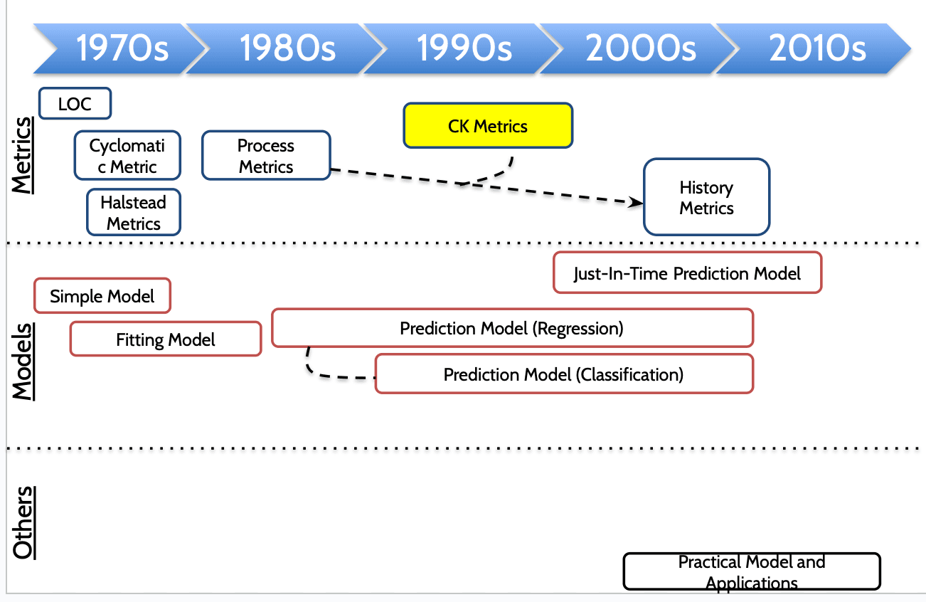
Representative OO Metrics대표적인 객체지향 메트릭

• CK metrics (Chidamber&Kemerer@TSE`94)CK 메트릭 (Chidamber & Kemerer, 1994)

• Prediction Performance of CK vs. code (Basili@TSE96)CK 메트릭 vs. 코드 메트릭의 예측 성능 비교 (Basili@TSE96)

  • F-measure: 70% vs. 60%F-점수: 70% (CK) vs. 60% (코드 메트릭)

Defect Prediction Approaches (7)결함 예측 접근 방식

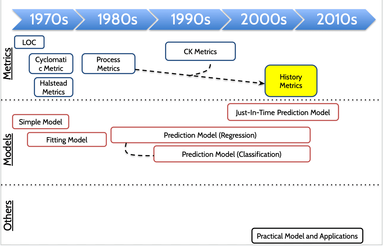
Representative History Metrics대표적인 히스토리 메트릭

• SW Repo. = version control system + issue tracking systemSW 저장소 = 버전 관리 시스템 + 이슈 추적 시스템

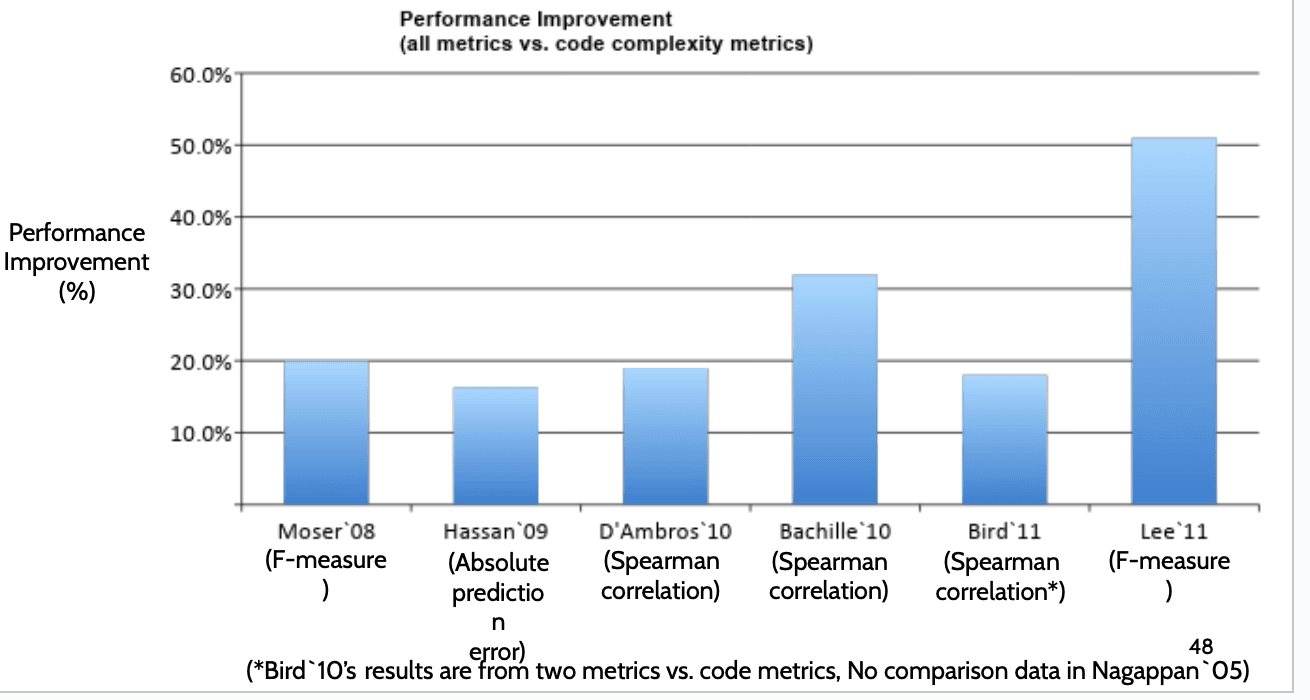
• Advantage장점

  • Better prediction performance than code metrics코드 메트릭보다 더 나은 예측 성능

History Metrics히스토리 메트릭

• Limitations제한 사항

  • History metrics do not extract particular program characteristics such as developer social network, component network, and anti-pattern.히스토리 메트릭은 개발자 소셜 네트워크, 컴포넌트 네트워크, 안티 패턴 같은 특정한 프로그램 특성을 추출하지 못한다.

  • Noise data노이즈 데이터 존재

    • Bias in Bug-Fix Dataset (Bird@FSE09)버그 수정 데이터셋에 편향 존재 (Bird@FSE09)

  • Not applicable for new projects and projects lacking in historical data신규 프로젝트나 히스토리 데이터가 부족한 프로젝트에는 적용 불가

Defect Prediction Approaches (8)결함 예측 접근 방식

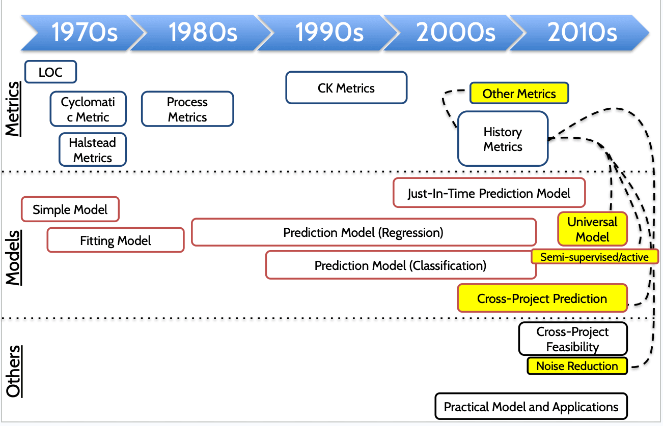
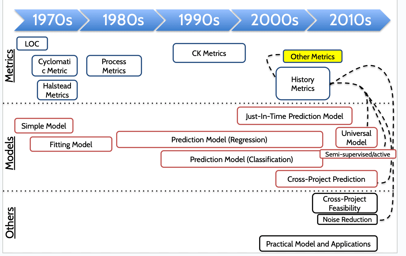
Other Metrics기타 메트릭

• SW Repo. = version control system + issue tracking systemSW 저장소 = 버전 관리 시스템 + 이슈 추적 시스템

Defect Prediction Approaches (9)결함 예측 접근 방식

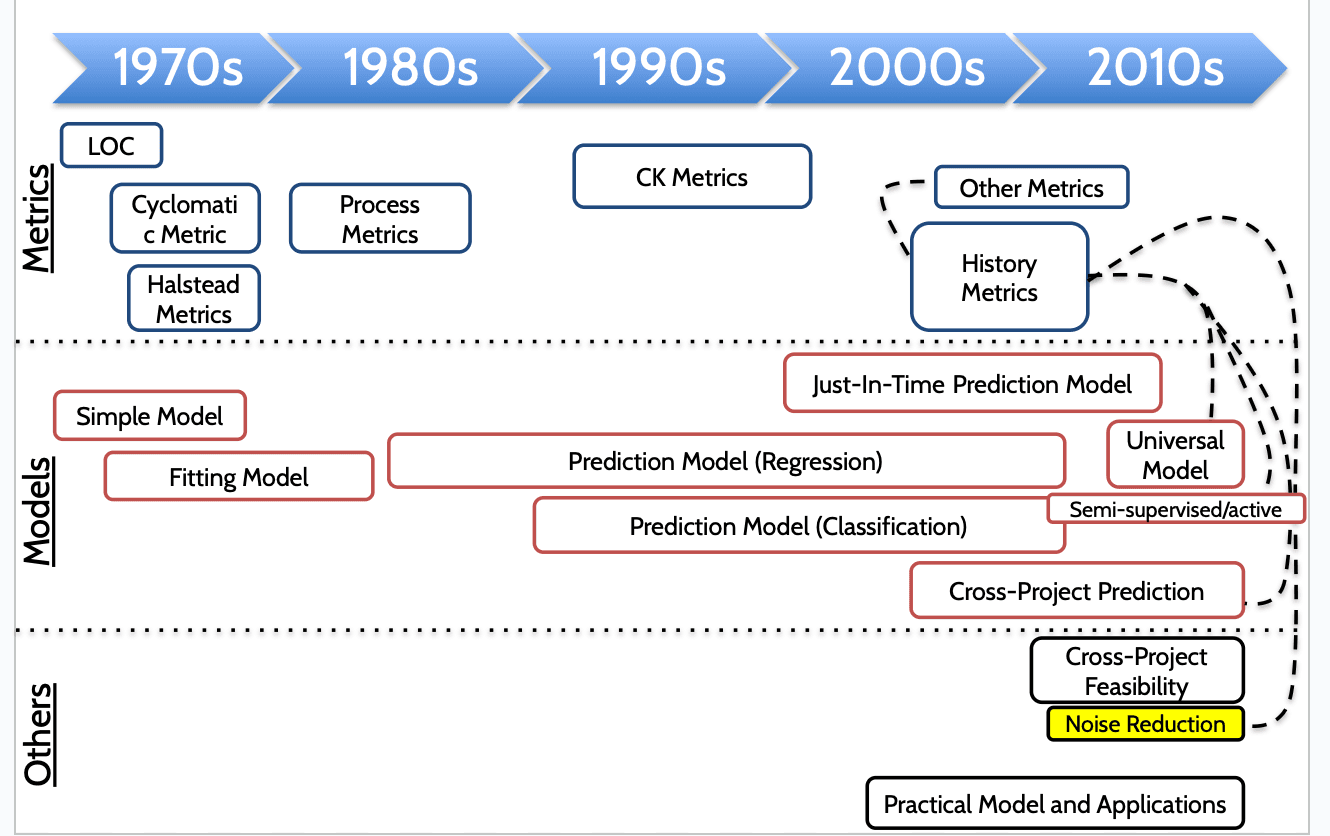
Noise Reduction노이즈 제거

• Noise detection and elimination algorithm (Kim@ICSE11) 노이즈 탐지 및 제거 알고리즘 (Kim@ICSE11)

  • Closest List Noise Identification (CLNI)CLNI 알고리즘

    • Based on Euclidean distance between instances인스턴스 간 유클리디안 거리 기반

  • Average F-measure improvement평균 F-점수 향상

    • 0.504 → 0.6210.504에서 0.621로 개선

• Relink (Wu@FSE11)ReLink 기법 (Wu@FSE11)

  • Recover missing links between bugs and commits버그와 커밋 간 누락된 연결 복원

  • 60% → 78% recall for missing links누락 링크에 대한 재현율 60% → 78%

  • F-measure improvementF-점수 향상

    • e.g. 0.698 (traditional) → 0.731 (ReLink)예: 기존 방식 0.698 → ReLink 0.731

Defect Prediction Approaches (10)결함 예측 접근 방식

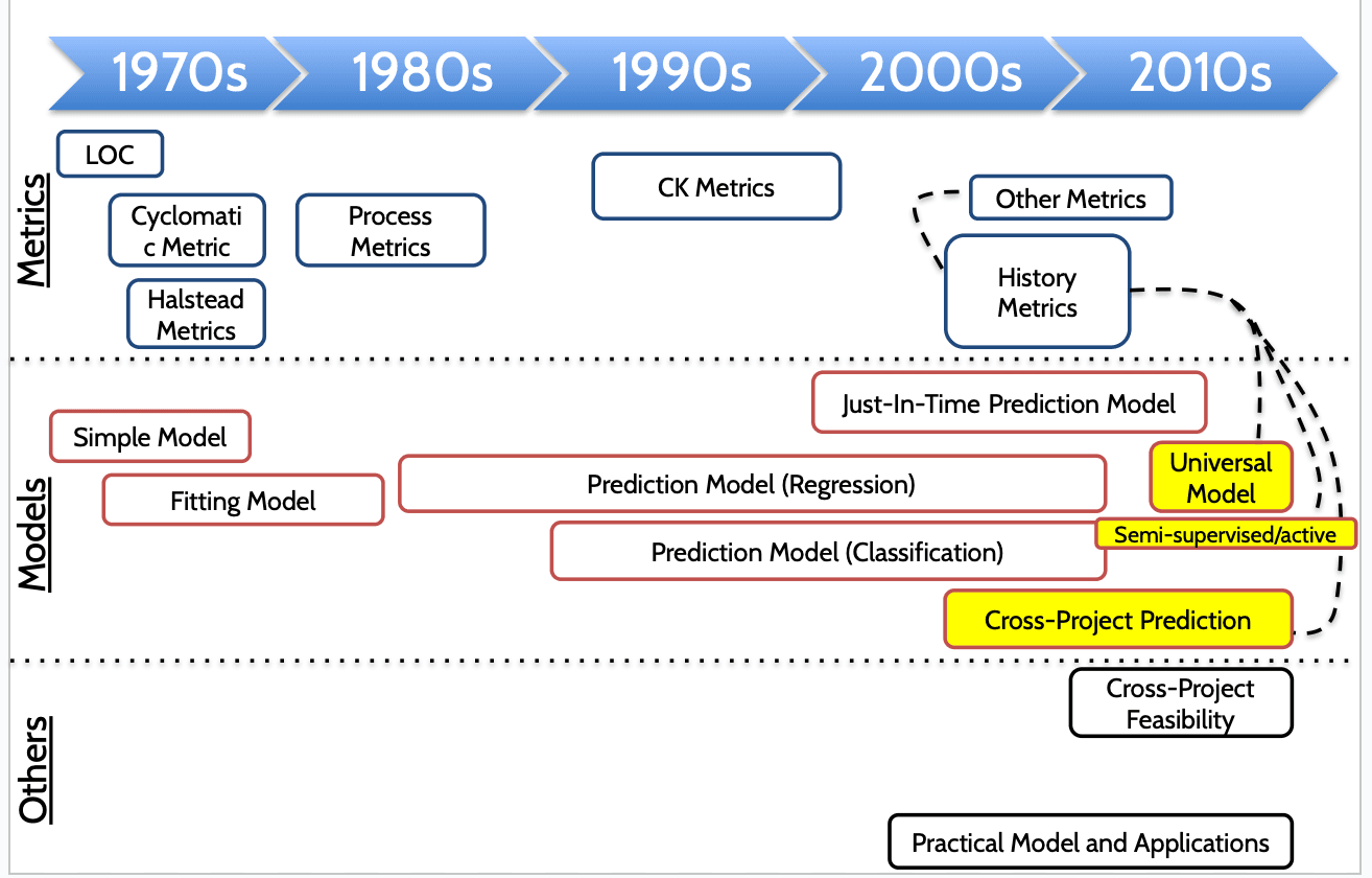
Defect Prediction for New Software Projects신규 소프트웨어 프로젝트를 위한 결함 예측

• Universal Defect Prediction Model범용 결함 예측 모델

• Semi-supervised / active learning준지도 학습 / 능동 학습

• Cross-Project Defect Prediction크로스 프로젝트 결함 예측 (CPDP)

Universal Defect Prediction Model (Zhang@MSR14) 범용 결함 예측 모델 (Zhang@MSR14)

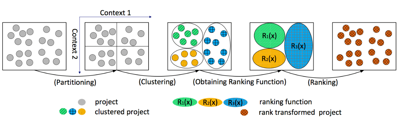
• Context-aware rank transformation컨텍스트 인식 순위 변환

  • Transform metric values ranged from 1 to 10 across all projects.모든 프로젝트에서 메트릭 값을 1~10 범위로 정규화

• Model built by 1398 projects collected from SourceForge and Google codeSourceForge와 Google Code에서 수집한 1,398개 프로젝트 기반 모델

Defect Prediction Approaches (11)결함 예측 접근 방식

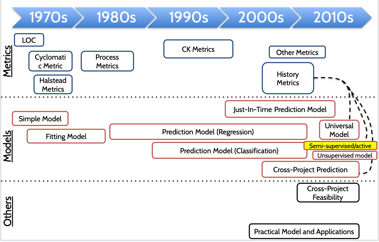
Semi-supervised/Active learning준지도 / 능동 학습

• Semi-supervised learning with dimension reduction for defect prediction (Lu@ASE12)결함 예측을 위한 차원 축소 기반 준지도 학습 (Lu@ASE12)

  • Training a model by a small set of labeled instances together with many unlabeled instances소수의 라벨링된 데이터와 다수의 비라벨 데이터로 모델 학습

  • AUC improvementAUC 향상

    • 0.83 → 0.88 with 2% labeled instances라벨링된 인스턴스가 2%일 때 AUC 0.83 → 0.88

• Sample-based semi-supervised/active learning for defect prediction (Li@AESEJ12)샘플 기반 준지도 / 능동 학습 (Li@AESEJ12)

  • Average F-measure평균 F-점수

    • 0.628 → 0.685 with 10% sampled instances샘플링 10%일 때 0.628 → 0.685

Defect Prediction Approaches (12)결함 예측 접근 방식

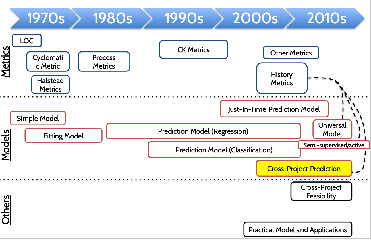
Cross-Project Defect Prediction (CPDP)크로스 프로젝트 결함 예측

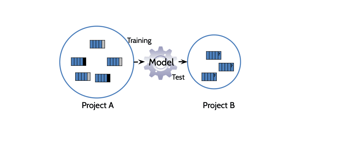
Transfer Learning (TL)전이 학습

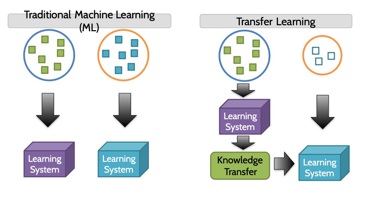
• Traditional Machine Learning (ML)전통적인 머신러닝

• Transfer Learning전이 학습

• Pan et al.@TNN`10, Domain Adaptation via Transfer Component Analysis도메인 적응 기반 전이 컴포넌트 분석 (Pan 외, 2010)

CPDP크로스 프로젝트 결함 예측

• Adopting transfer learning전이 학습을 도입함

Metric Compensation (Watanabe@PROMISE '08)메트릭 보상 (Watanabe@PROMISE '08)

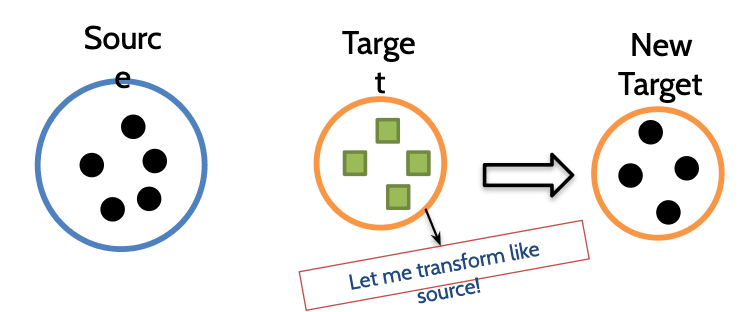
• Key idea핵심 아이디어

• New target metric value = target metric value × average source metric value / average target metric value새로운 타겟 메트릭 값 = 타겟 메트릭 값 × 소스 평균 메트릭 값 / 타겟 평균 메트릭 값

NN Filter (Turhan@ESEJ '09)최근접 이웃 필터 (Turhan@ESEJ '09)

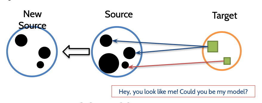
• Key idea핵심 아이디어

• Nearest neighbor filter최근접 이웃 필터 사용

  • Select 10 nearest source instances of each target instance각 타겟 인스턴스에 대해 가장 가까운 소스 인스턴스 10개를 선택

Transfer Naive Bayes (Ma@IST '12)전이 나이브 베이즈 (Ma@IST '12)

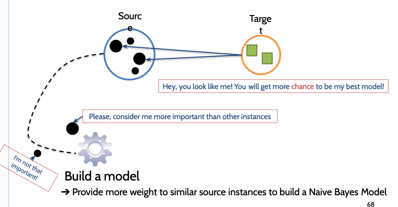
• Key idea핵심 아이디어

  • Build a model ➔ Provide more weight to similar source instances to build a Naive Bayes Model
    모델을 학습할 때, 유사한 소스 인스턴스에 더 많은 가중치를 부여하여 나이브 베이즈 모델 생성

Transfer Naive Bayes (cont.) (Ma@IST '12)전이 나이브 베이즈 (계속) (Ma@IST '12)

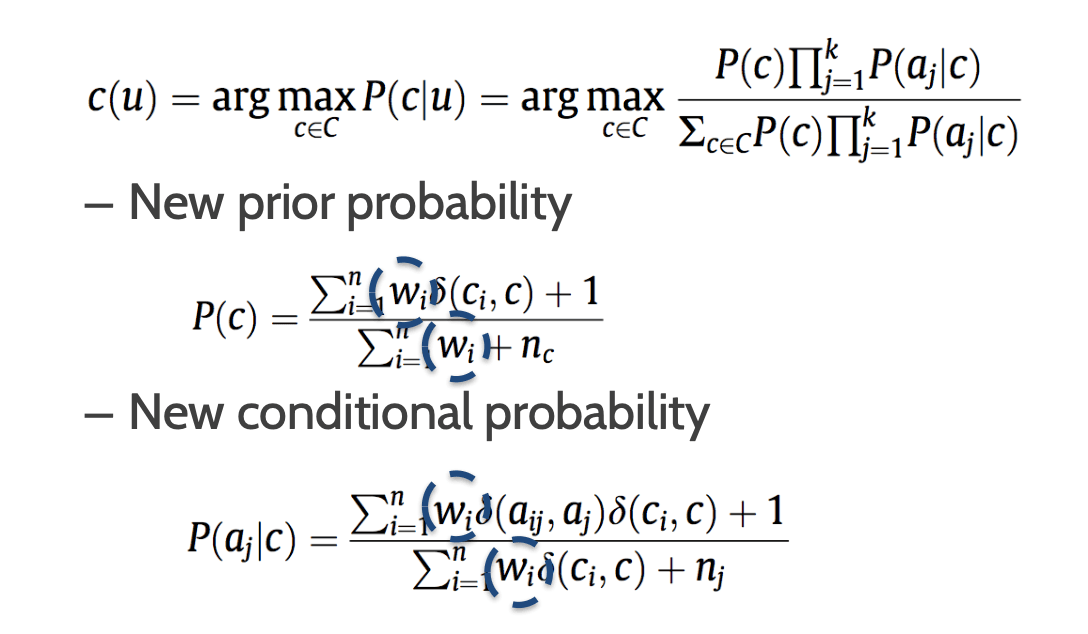
• Transfer Naive Bayes전이 기반 나이브 베이즈

  • New prior probability
    새로운 사전 확률 계산

  • New conditional probability
    새로운 조건부 확률 계산

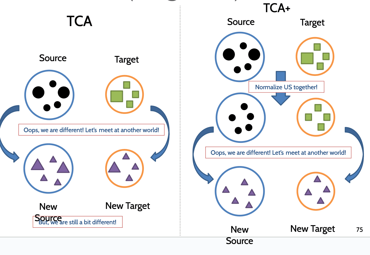
TCA+ (Nam@ICSE '13)

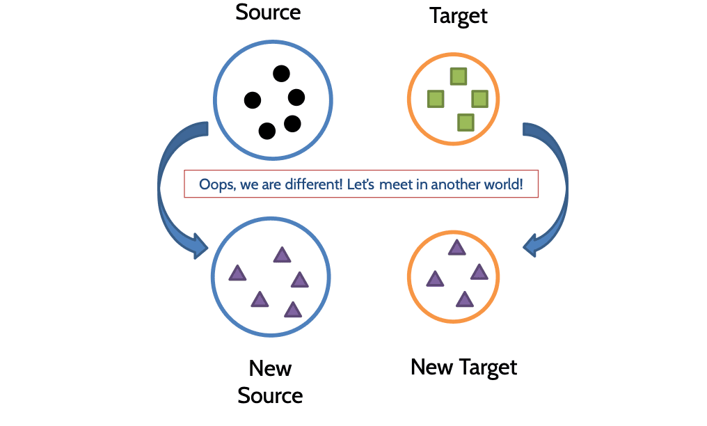
• Key idea핵심 아이디어

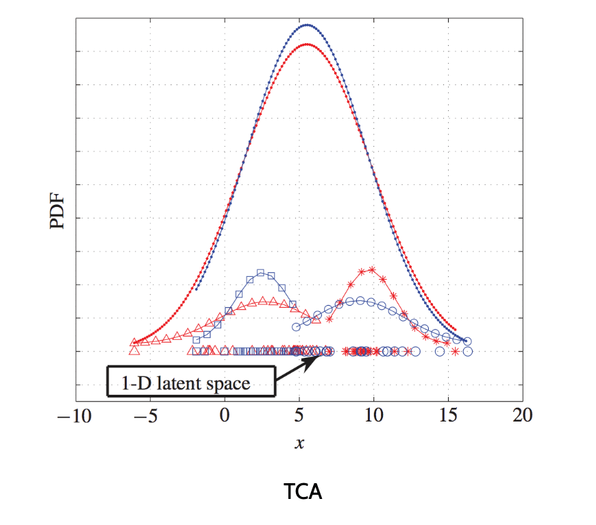
  • TCA (Transfer Component Analysis)
    TCA (전이 성분 분석) 기반 접근

Transfer Component Analysis (cont.)전이 성분 분석 (계속)

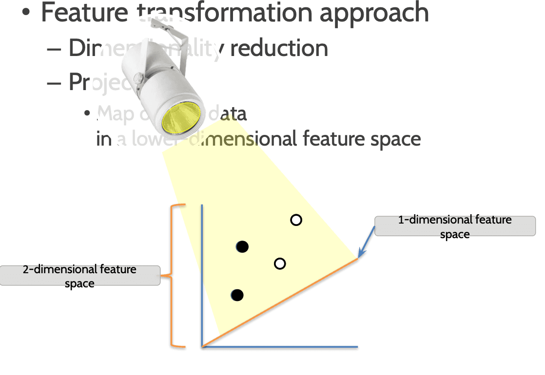
• Feature transformation approach특성 변환 방식 사용

  • Dimensionality reduction
    차원 축소 수행

  • Projection
    투영 기법 적용

    • Map original data in a lower-dimensional feature space
      원본 데이터를 저차원 특성 공간에 매핑

TCA (cont)

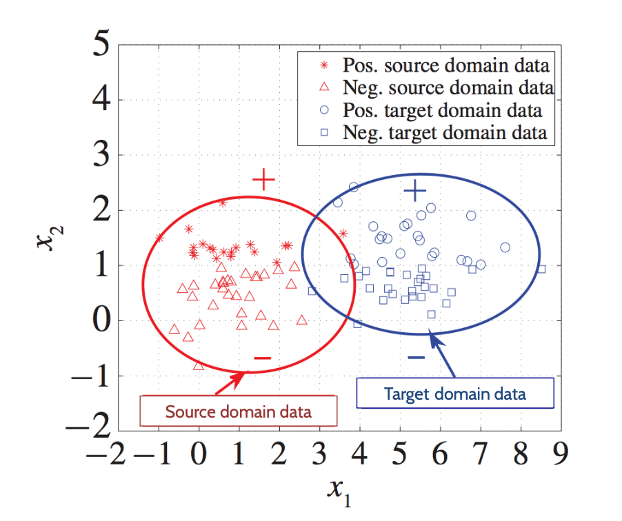
TCA+ (Nam@ICSE'13)

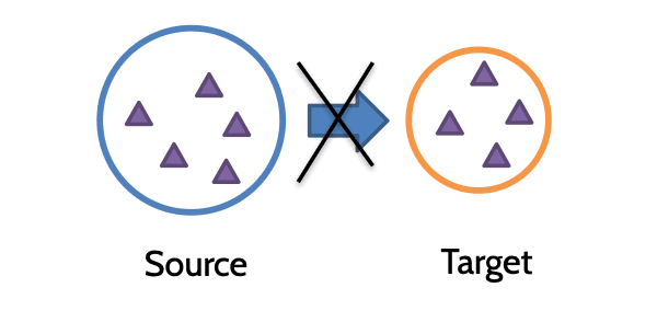
Current CPDP using TL전이 학습을 활용한 현재의 크로스 프로젝트 결함 예측 (CPDP)

• Advantages장점

  • Comparable prediction performance to within-prediction models동일 프로젝트 내 예측 모델과 유사한 성능을 보임

  • Benefit from the state-of-the-art TL approaches최신 전이 학습 기법의 이점을 활용함

• Limitation한계

  • Performance of some cross-prediction pairs is still poor. (Negative Transfer)일부 크로스 예측 쌍에서는 여전히 성능이 낮음 (부정적 전이)

Defect Prediction Approaches (13)결함 예측 접근 방식

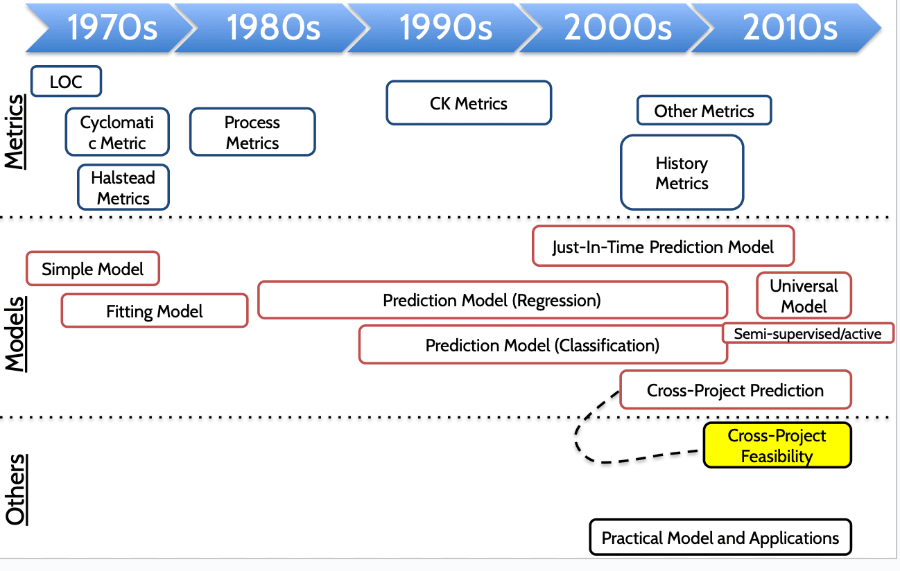
Feasibility Evaluation for CPDPCPDP의 적용 가능성 평가

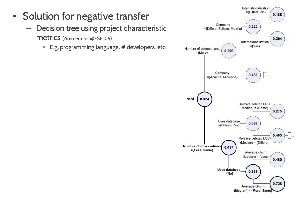
• Solution for negative transfer부정적 전이 문제 해결 방안

  • Decision tree using project characteristic metrics (Zimmermann@FSE`09)프로젝트 특성 메트릭을 이용한 결정 트리

    • E.g. programming language, # developers, etc.예: 프로그래밍 언어, 개발자 수 등

Follow-up Studies후속 연구들

• “An investigation on the feasibility of cross-project defect prediction.” (He@ASEJ12)크로스 프로젝트 결함 예측 가능성에 대한 조사 (He@ASEJ12)

  • Decision tree using distributional characteristics of a dataset데이터셋의 분포 특성(평균, 왜도, 첨도 등)을 이용한 결정 트리

Defect Prediction Approaches (14)결함 예측 접근 방식

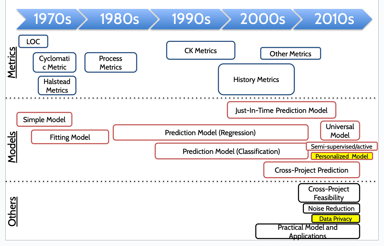
Other Topics기타 주제들

• Privacy issue on defect datasets결함 데이터셋의 개인정보 문제

  • MORPH (Peters@ICSE12)MORPH 기법 (Peters@ICSE12)

    • Mutate defect datasets while keeping prediction accuracy예측 정확도를 유지하면서 데이터셋을 변형함

    • Can accelerate cross-project defect prediction with industrial datasets산업용 데이터셋에서의 CPDP를 촉진할 수 있음

• Personalized defect prediction model (Jiang@ASE13)개인화된 결함 예측 모델 (Jiang@ASE13)

  • “Different developers have different coding styles, commit frequencies, and experience levels, all of which cause different defect patterns.”"개발자는 코딩 스타일, 커밋 빈도, 경험 수준이 다르며, 이는 각기 다른 결함 패턴을 유발한다."

  • Results결과

    • Average F-measure: 0.62 (personalized models) vs. 0.59 (non-personalized models)평균 F-점수: 개인화 모델 0.62 vs. 비개인화 모델 0.59

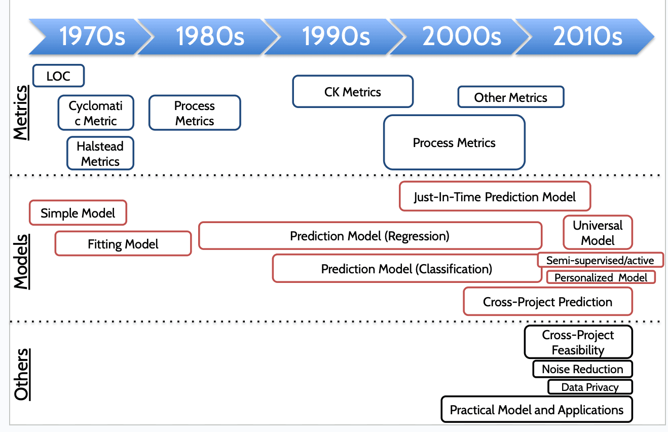
Defect Prediction Approaches (15)결함 예측 접근 방식

Agenda

• Problem definition
  문제 정의

• Defect prediction process based on machine learning머신러닝 기반 결함 예측 과정

• History of defect prediction studies결함 예측 연구의 역사

• Recent research trends최근 연구 동향

• Current challenges현재의 도전 과제

Recent research trends최근 연구 동향

• Heterogeneous Defect Prediction이질적인 결함 예측

• Unsupervised learning based Defect Prediction비지도 학습 기반 결함 예측

• Deep-learning based Defect Prediction Techniques딥러닝 기반 결함 예측 기법

Current Defect Prediction Studies현재 결함 예측 연구

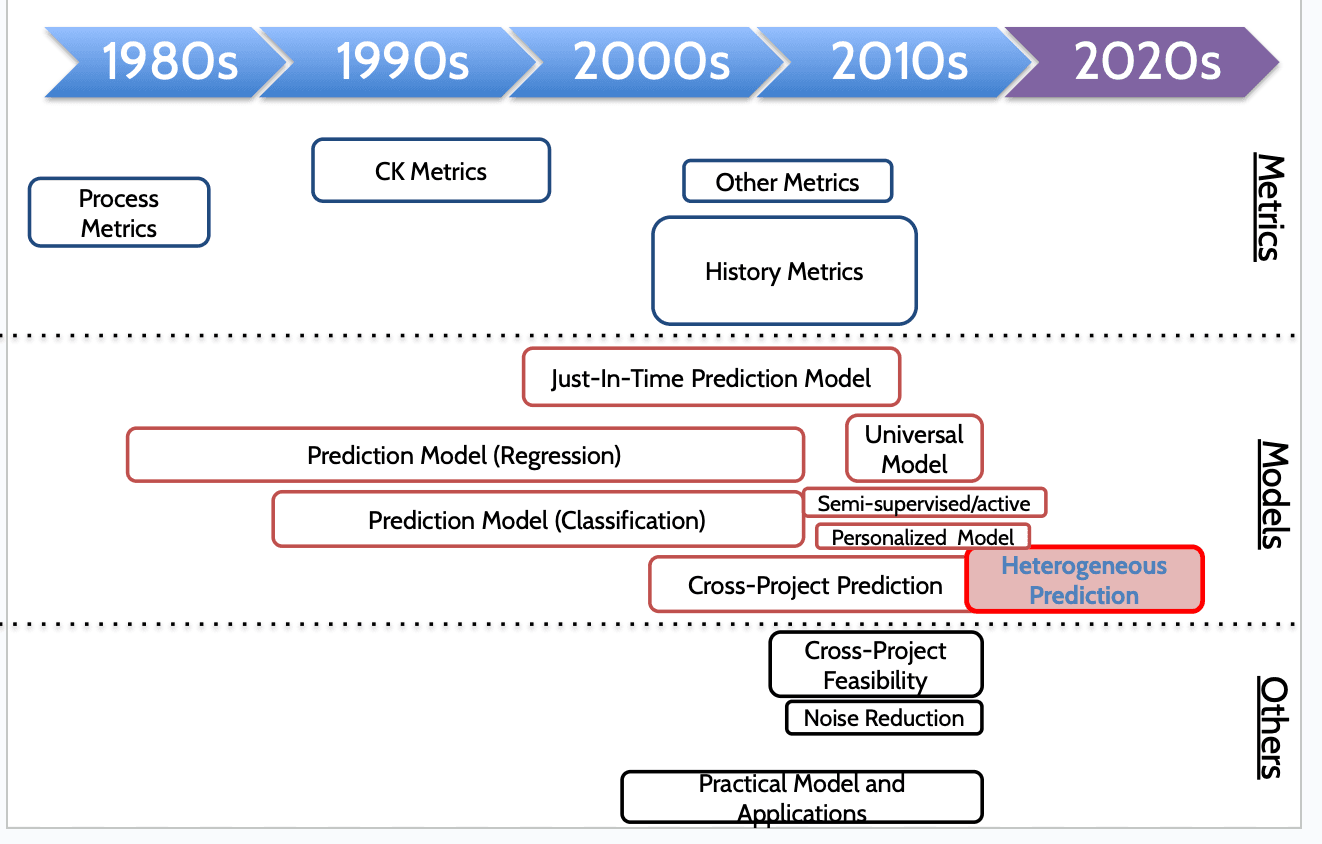
Cross-prediction Model크로스 예측 모델

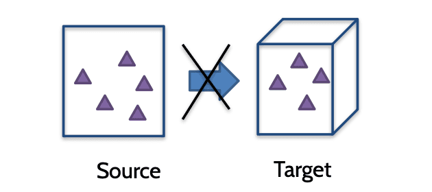
• Common challenge공통된 도전 과제

  • Current cross-prediction models are limited to datasets with same number of metrics현재의 모델은 동일한 메트릭 수를 가진 데이터셋에만 적용 가능

  • Not applicable on projects with different feature spaces (different domains)다른 특성 공간(도메인)을 가진 프로젝트에는 적용 불가

    • NASA Dataset: Halstead, LOCNASA 데이터셋: Halstead, LOC

    • Apache Dataset: LOC, Cyclomatic, CK metricsApache 데이터셋: LOC, 사이클로매틱, CK 메트릭

• Heterogeneous Defect Prediction (Nam@FSE15)

• 이질적 결함 예측 (Nam@FSE15)

Heterogeneous Defect Prediction이질적인 결함 예측

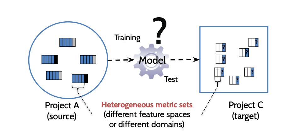
• Heterogeneous metric sets이질적인 메트릭 집합

  • (different feature spaces or different domains)(서로 다른 특성 공간 또는 도메인)

• Heterogeneous Defect Prediction (HDP)이질적 결함 예측 (HDP)

• Possible to Reuse all the existing defect datasets for CPDP!모든 기존 결함 데이터셋을 CPDP에 재사용할 수 있음!

Heterogeneous Defect Prediction이질적인 결함 예측

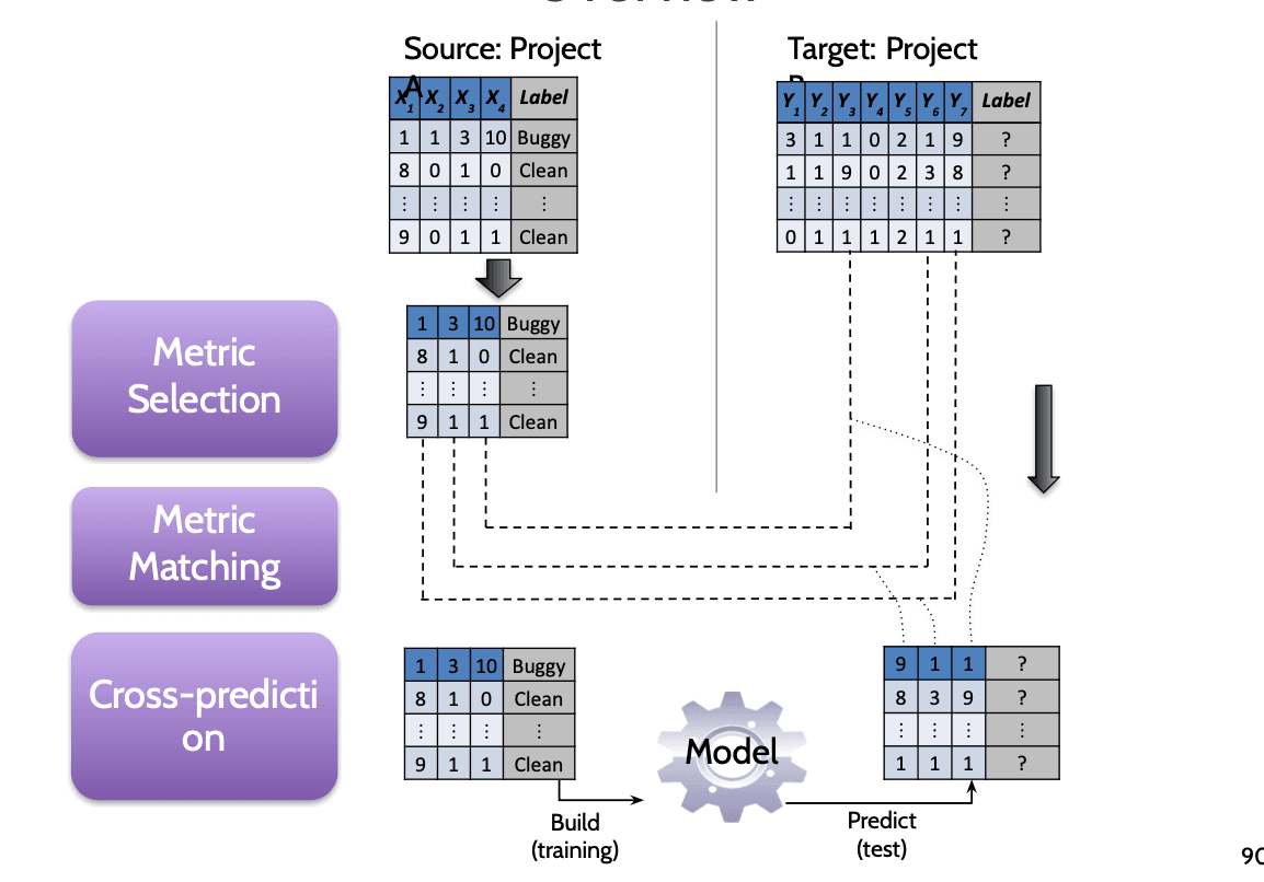
• Key Idea핵심 아이디어

• Most defect prediction metrics대부분의 결함 예측 메트릭은

  • Measure complexity of software and its development process.소프트웨어 및 개발 과정의 복잡도를 측정함

    • e.g.

      • The number of developers touching a source code file (Bird@FSE11)소스코드 파일을 수정한 개발자 수

      • The number of methods in a class (D’Ambroas@ESEJ12)클래스 내 메서드 수

      • The number of operands (Menzies@TSE`08)피연산자 수

  • More complexity implies more defect-proneness (Rahman@ICSE13)더 복잡할수록 결함 발생 가능성이 높다 (Rahman@ICSE13)

• Match source and target metrics that have similar distribution소스 및 대상 메트릭의 분포가 유사한 경우 일치시키기

Compute Matching Score KSAnalyzerKSAnalyzer를 통한 매칭 점수 계산

• Use p-value of Kolmogorov-Smirnov Test (Massey@JASA`51)Kolmogorov-Smirnov 검정의 p-값을 사용함

• Matching Score M of i-th source and j-th target metrics: M_ip = p_iji번째 소스와 j번째 대상의 매칭 점수 M: M_ip = p_ij

Matched Metrics매칭된 메트릭

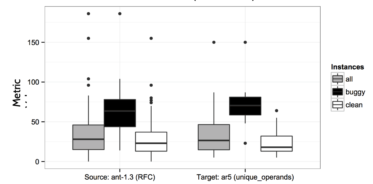
• AUC = 0.946 (ant1.3 → ar5)

• Distribution

  • (Source metric: RFC - 클래스에서 호출된 메서드 수, Target metric: 피연산자 수)

• Matching Score = 0.91매칭 점수 = 0.91

Prediction Results in median AUC

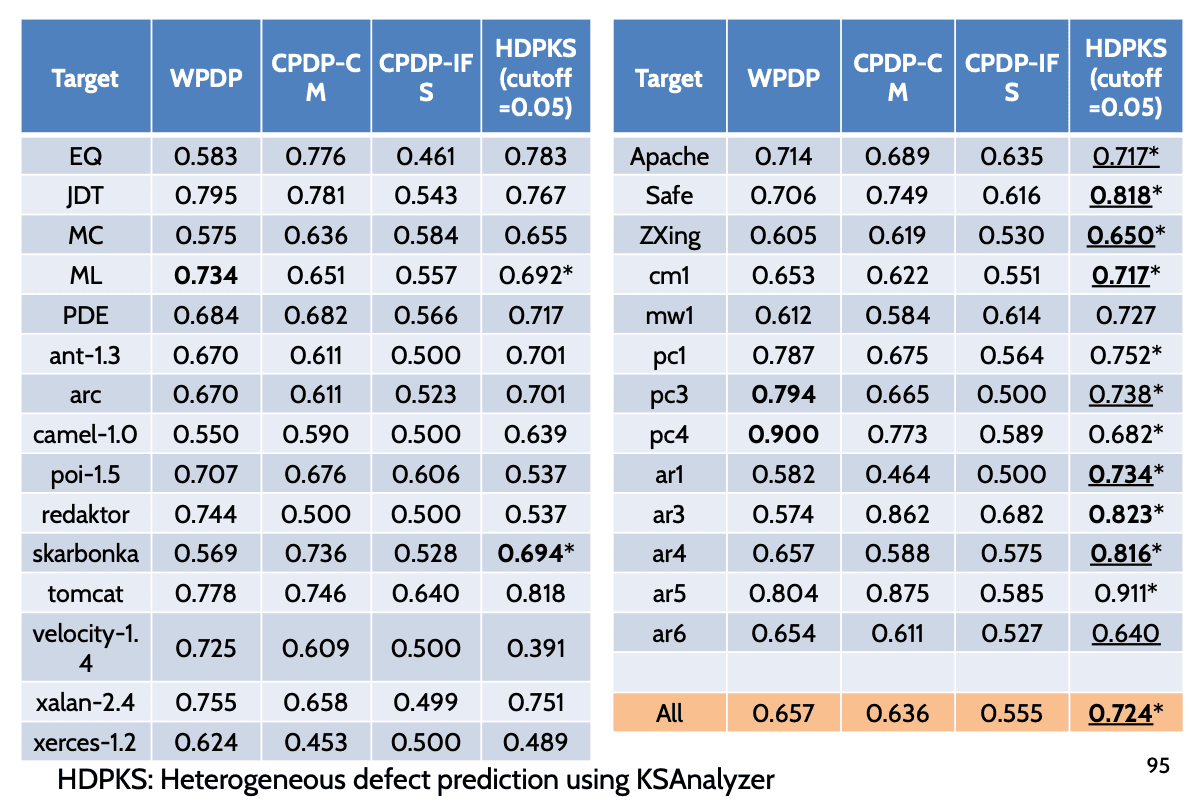
Current Defect Prediction Studies현재 결함 예측 연구

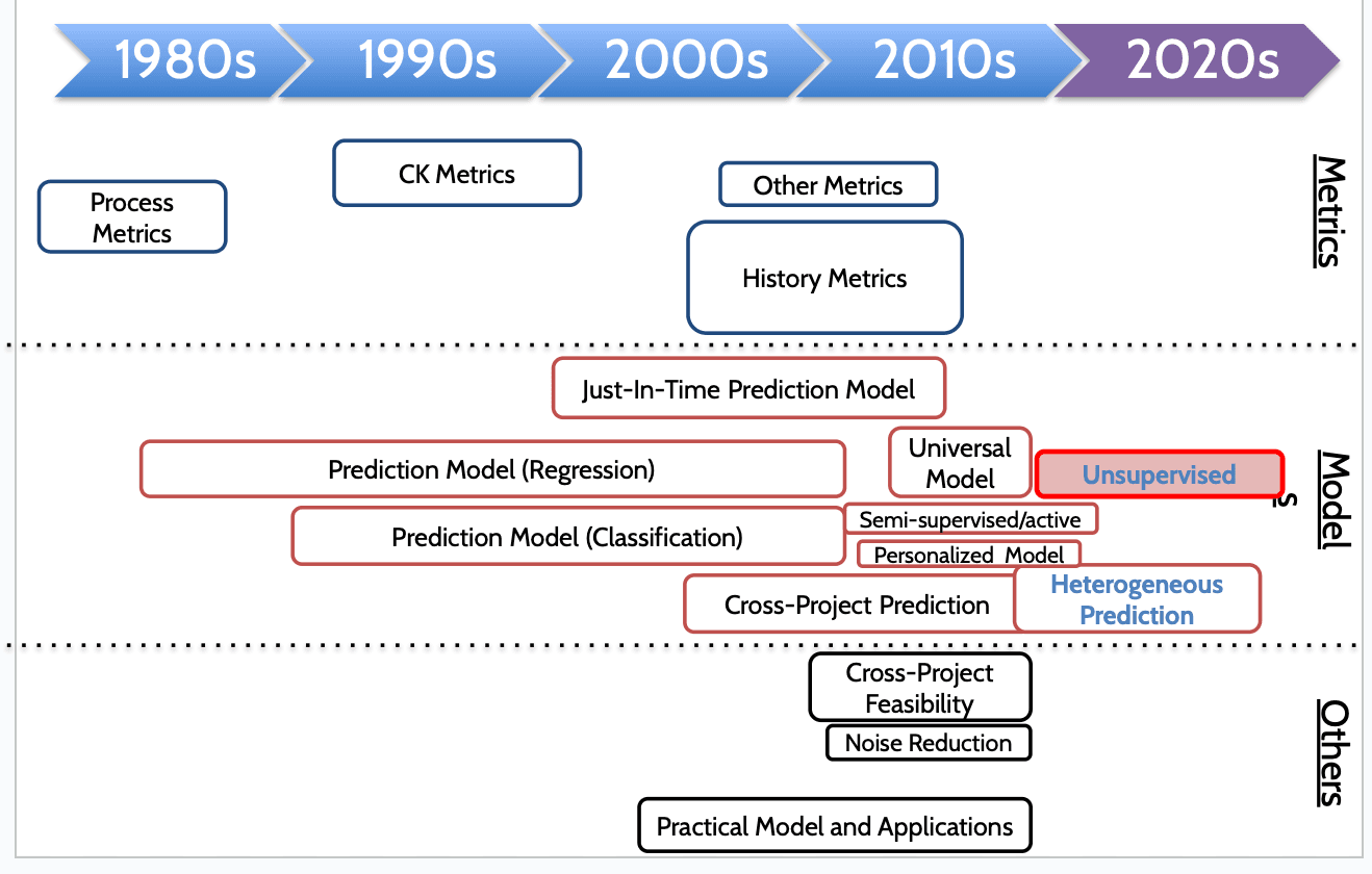
Unsupervised learning based Defect Prediction비지도 학습 기반 결함 예측

• CLAMI (Nam et al.@ASE 2015)CLAMI (남 등, ASE 2015)

• Connectivity-based Unsupervised Classifier (Zhang et al.@ICSE 2016)연결성 기반 비지도 분류기 (장 등, ICSE 2016)

CLA/CLAMI Approach OverviewCLA/CLAMI 접근법 개요

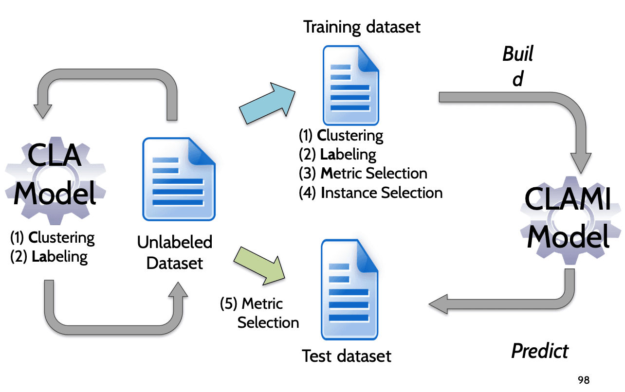
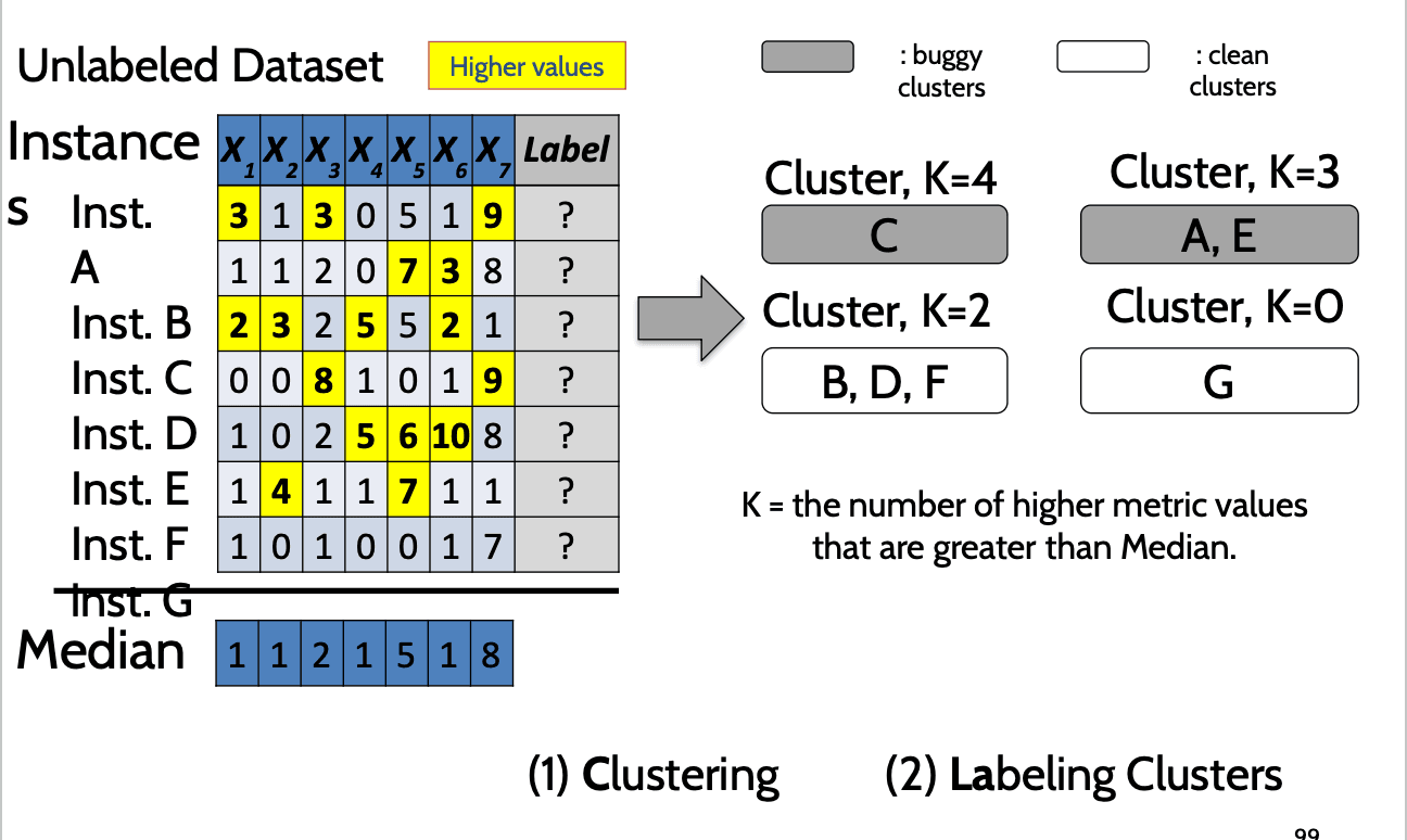
CLAM/CLAMI Approach - Clustering and Labeling Clusters -CLA/CLAMI 접근 방식 - 클러스터링 및 클러스터에 라벨링

CLAM/CLAMI Approach - Metric SelectionCLAM/CLAMI 접근 방식 - 메트릭 선택

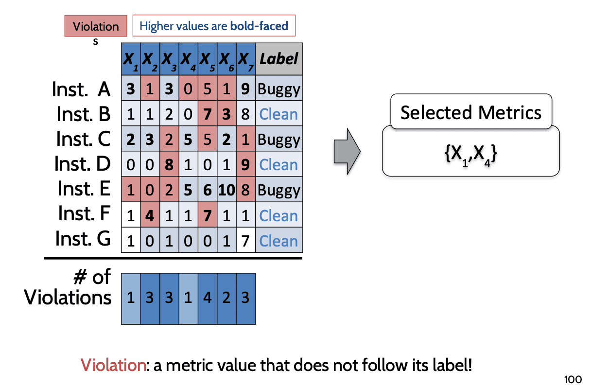
• Violation: a metric value that does not follow its label!위반: 라벨과 일치하지 않는 메트릭 값!

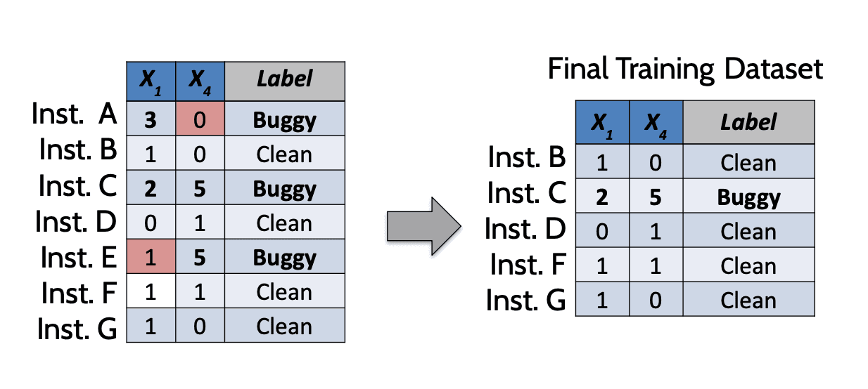
CLAMI Approach - Instance Selection -CLAMI 접근법 - 인스턴스 선택 -

CLAMI: F-measure and AUCCLAMI: F-측정값과 AUC

• Wilcoxon Signed-Rank Test for Each Project각 프로젝트에 대한 Wilcoxon 부호순위 검정

• SL (Supervised Learning) vs CLA/CLAMI: BoldSL (지도 학습) vs CLA/CLAMI: 굵은 글씨

• THD (Threshold-based) vs CLA/CLAMI: BlueTHD (임계값 기반) vs CLA/CLAMI: 파란색 표시

• **EXP (Expert-based) vs CLA/CLAMI: ***EXP (전문가 기반) vs CLA/CLAMI: 별표 표시

• CLA vs CLAMI: _____CLA vs CLAMI: 밑줄 표시

CLAMI: Distributions of metrics (Safe)

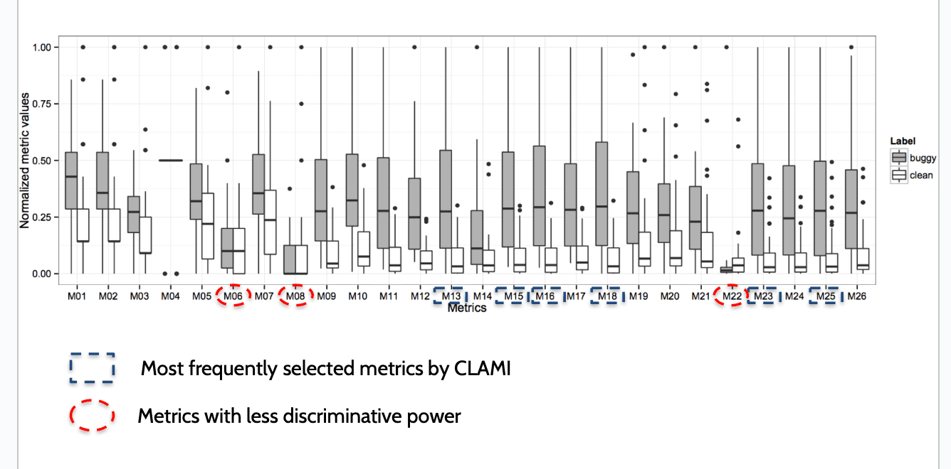
• Most frequently selected metrics by CLAMICLAMI에 의해 가장 자주 선택된 메트릭들

• Metrics with less discriminative power구분력이 낮은 메트릭들

Current Defect Prediction Studies현재 결함 예측 연구 동향

Deep learning based Defect Prediction딥러닝 기반 결함 예측

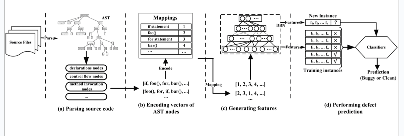
• Semantic Feature Generation Using Deep Belief Network (Wang et al.@ICSE 2016)딥 빌리프 네트워크를 활용한 의미 기반 특성 생성 (Wang 외, ICSE 2016)

Deep learning is Necessary?딥러닝이 반드시 필요한가?

• Easy over Hard: A Case Study on Deep Learning (Fu et al.@FSE 2017)쉬운 방법이 어려운 방법보다 나은가: 딥러닝 사례 연구 (Fu 외, FSE 2017)

  • Deep Learning딥러닝

    • Highly computationally expensive (days to weeks)계산 비용이 매우 크다 (수일에서 수주 소요)

  • What if simple and fast methods can achieve the comparable results to the results of deep learning approach??간단하고 빠른 방법이 딥러닝과 유사한 결과를 낼 수 있다면?

    • Parameter tuning하이퍼파라미터 조정

    • Understand a task and match a technology wisely과제를 이해하고 적절한 기술을 현명하게 선택하라

Agenda

• Problem definition
  문제 정의

• Defect prediction process based on machine learning머신러닝 기반 결함 예측 과정

• History of defect prediction studies결함 예측 연구의 역사

• Recent research trends최근 연구 동향

• Current challenges현재의 도전 과제

Next Steps of Defect Prediction결함 예측의 다음 단계